Simple explanation for Capsule Network with Pytoch implementation

15 minute read

Capsule Network

In this blog post i will try to explain and implement Capsule Networks on MNIST images using Pytorch.

To implement capsule Network, we need to understand what are capsules first and what advantages do they have compared to convolutional neural network.

what are capsules?

Briefly explaining it, capsules are small group of neurons where each neuron in a capsule represents various properties of a particular image part.
Capsules represent relationships between parts of a whole object by using dynamic routing to weight the connections between one layer of capsules and the next and creating strong connections between spatially-related object parts, will be discussed later.
The output of each capsule is a vector, this vector has a magnitude and orientation.
- Magnitude : It is an indicates if that particular part of image is present or not. Basically we can summerize it as the probability of the part existance (It has to be between 0 and 1).
- Oriantation : It changes if one of the properties of that particular image has changed.
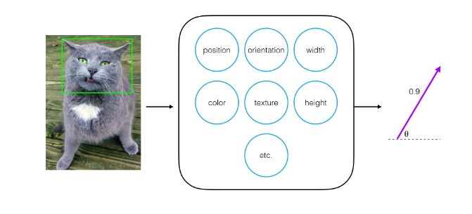
Let us have an example to understand it more and make it clear. As shown in the following image, capsules will detect a cat’s face. As shown in the image the capsule consists of neurals with properties like the position,color,width and etc.. .Then we get a vector output with magnitude 0.9 which means we have 90% confidence that this is a cat face and we will get an orientation as well.

/recon_cover.png image from :cezannec’s blog

But what if we have changed in these properties like we have flipped the cat’s face,what will happen ? will it detect the cat face? Yes it still will detect the cat’s face with 90% confidance(with magnitude 0.9) but there will be a change in the oriantation(theta)to indicate a change in the properties.

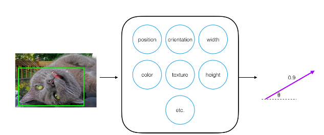image from :cezannec’s blog

What advantages does it have compared to Convolutional Neural Network(CNN)?

CNN is looking for key features regadless their position. As shown in the following image, CNN will detect the left image as a face while capsule network will not detect them as it will check if they are in the correct postition or not.

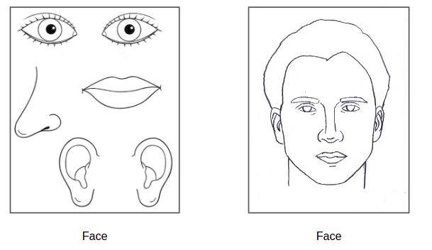image from :kndrck’s blog
Capsules network is more rubust to affine transformations in data. If translation or rotation is done on test data, a trained Capsule network will preform better and will give a higher accuracy than normal CNN.

Model Architecture

The capsule network is consisting of two main parts:

A convolutional encoder.
A fully connected, linear decoder.

alt

(image from :Hinton’s paper(capsule networks orignal paper) )

In this Explantaion and implementation i will follow the architecture from Hinton paper(capsule networks orignal paper)

1)Encoder

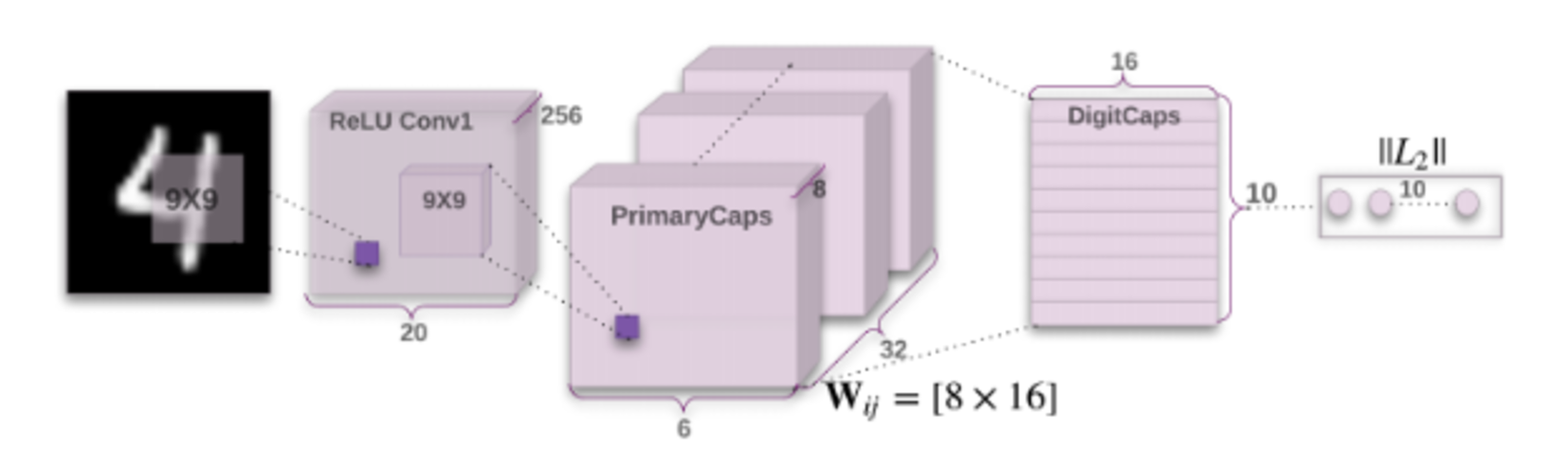
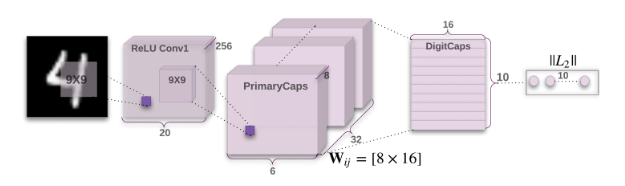
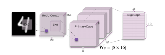
The ecnoder consists of three main layers as shown in the following image and the input layer which is from MNIST which has a dimension of 28 x28.

please notice the difference between this image and the previous image where the last layer is the decoder in the pravious image.

alt

A)The convolutional layer

So in Hinton’s paper they have applied a kernel of size 9x9 to the input layer. This kernel has a depth of 256,stride =1 and padding = 0.This will give us an output of a dimenstion 20x20.

Note : you can calculate the output dimenstion by this eqaution, output = [(w-k+2p)/s]+1 , where:

w is the input size
k is the kernel size
p is padding
s is stride

So to clarify this more:

The input’s dimension is (28,28,1) where the 28x28 is the input size and 1 is the number of channels.
Kernel’s dimention is (9,9,1,256) where 9x9 is the kernel size ,1 is the number of channels and 256 is the depth of the kernel .
The output’s dimension is (20,20,256) where 20x20 is the ouptut size and 256 is the stack of filtered images.

I think we are ready to start implementing the code now, so let us start by obtaining the MNIST data and create our DataLoaders for training and testing purposes.

    from torchvision import datasets
    import torchvision.transforms as transforms

    # number of subprocesses to use for data loading
    num_workers = 0
    # how many samples per batch to load
    batch_size = 20

    # convert data to Tensors
    transform = transforms.ToTensor()

    # choose the training and test datasets
    train_data = datasets.MNIST(root='data', train=True,
                                download=True, transform=transform)

    test_data = datasets.MNIST(root='data', train=False,
                               download=True, transform=transform)

    # prepare data loaders
    train_loader = torch.utils.data.DataLoader(train_data,
                                               batch_size=batch_size,
                                               num_workers=num_workers)

    test_loader = torch.utils.data.DataLoader(test_data,
                                              batch_size=batch_size,
                                              num_workers=num_workers)

The nexts step is to create the convolutional layer as we explained:

    class ConvLayer(nn.Module):

        def __init__(self, in_channels=1, out_channels=256):
            '''Constructs the ConvLayer with a specified input and output size.
               These sizes has initial values from the paper.
               param input_channel: input depth of an image, default value = 1
               param output_channel: output depth of the convolutional layer, default value = 256
               '''
            super(ConvLayer, self).__init__()

            # defining a convolutional layer of the specified size
            self.conv = nn.Conv2d(in_channels, out_channels,
                                  kernel_size=9, stride=1, padding=0)

        def forward(self, x):

            # applying a ReLu activation to the outputs of the conv layer
            output = F.relu(self.conv(x)) # we will have dimensions (batch_size, 20, 20, 256)
            return output

B)Primary capsules

This layer is tricky but i will try to simplify it as much as i can. We would like to convolute the first layer to a new layer with 8 primary capsules. To do so we will follow Hinton’s paper steps:

First step is to convolute our first Convolutional layer which has a dimension of (20 ,20 ,256) with a kernel of dimension(9,9,256,256) in which 9 is the kernel size,first 256 is the number of chanels from the first layer and the second 256 is the number of filters or the depth of the kernel.We will get an output with a dimension of (6,6,256) .
second step is to reshape this output to (6,6,8,32) where 8 is the number of capsules and 32 is the depth of each capsule .
Now the output of each capsule will have a dimension of (6,6,32) and we will reshape it to (32x32x6,1) = (1152,1) for each capsule.
Final step we will squash the output to have a magnitute between 0 and 1 as we have discussed earlier using the following equation :

\[v_j = \frac{||\ s_j^2\ ||\ s_j }{1 + ||\ s_j^2\ ||\ s_j }\]

where Vj is the normalized output vector of capsule j, Sj is the total inputs of each capsule (which is the sum of weights over all the output vectors from the capsules in the layer below capsule).

We will use ModuleList container to loop on each capsule we have.

    class PrimaryCaps(nn.Module):

        def __init__(self, num_capsules=8, in_channels=256, out_channels=32):
            '''Constructs a list of convolutional layers to be used in
               creating capsule output vectors.
               param num_capsules: number of capsules to create
               param in_channels: input depth of features, default value = 256
               param out_channels: output depth of the convolutional layers, default value = 32
               '''
            super(PrimaryCaps, self).__init__()

            # creating a list of convolutional layers for each capsule I want to create
            # all capsules have a conv layer with the same parameters
            self.capsules = nn.ModuleList([
                nn.Conv2d(in_channels=in_channels, out_channels=out_channels,
                          kernel_size=9, stride=2, padding=0)
                for _ in range(num_capsules)])

        def forward(self, x):
            '''Defines the feedforward behavior.
               param x: the input; features from a convolutional layer
               return: a set of normalized, capsule output vectors
               '''
            # get batch size of inputs
            batch_size = x.size(0)
            # reshape convolutional layer outputs to be (batch_size, vector_dim=1152, 1)
            u = [capsule(x).view(batch_size, 32 * 6 * 6, 1) for capsule in self.capsules]
            # stack up output vectors, u, one for each capsule
            u = torch.cat(u, dim=-1)
            # squashing the stack of vectors
            u_squash = self.squash(u)
            return u_squash

        def squash(self, input_tensor):
            '''Squashes an input Tensor so it has a magnitude between 0-1.
               param input_tensor: a stack of capsule inputs, s_j
               return: a stack of normalized, capsule output vectors, v_j
               '''
            squared_norm = (input_tensor ** 2).sum(dim=-1, keepdim=True)
            scale = squared_norm / (1 + squared_norm) # normalization coeff
            output_tensor = scale * input_tensor / torch.sqrt(squared_norm)    
            return output_tensor

C)Digit Capsules

As we have 10 digit classes from 0 to 9, this layer will have 10 capsules each capsule is for one digit. Each capsule takes an input of a batch of 1152 dimensional vector while the output is a ten 16 dimnsional vector.

Dynamic Routing

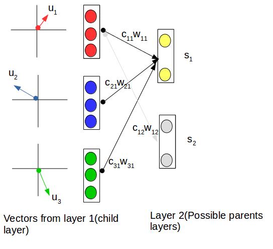
Dynamic routing is used to find the best matching between the best connections between the child layer and the possible parent.Main companents of the dynamic routing is the capsule routing. To make it easier we can think of the capsule routing as it is backprobagation.we can use it to obtain the probability that a certain capsule’s output should go to a parent capsule in the next layer.

As shown in the following figure The first child capsule is connected to \(s_{1}\) which is the fist possible parent capsule and to \(s_{2}\) which is the second possible parent capsule.In the begining the coupling will have equal values like both of them are zeros then we start apply dynamic routing to adjust it.We will find for example that coupling coffecient connected with \(s_{1}\) is 0.9 and coupling coffecient connected with \(s_{2}\) is 0.1, that means the probability that first child capsule’s output should go to a parent capsule in the next layer.

image-center

Notes

Across all connections between one child capsule and all possible parent capsules, the coupling coefficients should sum to 1.This means That \(c_{11}\) + \(c_{12}\) = 1 .
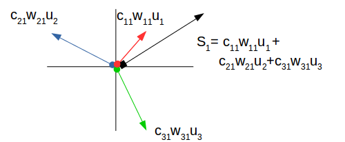
As shown in the following figure \(s_{1}\) is the total inputs of each capsule (which is the sum of weights over all the output vectors from the capsules in the layer below capsule).
To check the similarity between the total inputs \(s_{1}\) and each vector we will calculate the dot product between both of them, in this example we will find that \(s_{1}\) is more similar to \(u_{1}\) than \(u_{2}\) or \(u_{3}\) , This similarity called (agreement).

Dynamic Routing Algorithm

The followin algorithm is from Hinton’s paper(capsule networks orignal paper).

alt

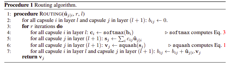
we can simply explain the algorithm as folowing :

First we initialize the initial logits \(b_{ij}\) of the softmax function with zero
calculate the capsule coefficiant using the softmax equation. \(c_{ij} = \frac{e^{\ b_{ij}}}{\sum_{k}\ {e^{\ b_{ik}}}}\)
calculate the total capsule inputs \(s_{1}\) .
squash to get a normalized vector output \(v_{j}\)
last step is composed of two steps, we will calculate agreement and the new \(b_{ij}\) .The similarity (agremeent) is that we have discussed before,which is the cross product between prediction vector \(\hat{u}\) and parent capsule’s output vector \(s_{1}\) . The second step is to update \(b_{ij}\) .

\[\hat{u} = W u\] \[a = v \cdot u\] \[b_{ij} = b_{ij} + a\]

Note

The equation of \(s_{j}\) is \(s_j = \sum{c_{ij} \ \hat{u}}\)
\(\hat{u} = Wu\) where W is the weight matrix and u is the input vector

Before implementing the Dynamic Routing we will transpose softmax function:

    def softmax(input_tensor, dim=1): # to get transpose softmax function # for multiplication reason s_J
        # transpose input
        transposed_input = input_tensor.transpose(dim, len(input_tensor.size()) - 1)
        # calculate softmax
        softmaxed_output = F.softmax(transposed_input.contiguous().view(-1, transposed_input.size(-1)), dim=-1)
        # un-transpose result
        return softmaxed_output.view(*transposed_input.size()).transpose(dim, len(input_tensor.size()) - 1)

After understanding the algorithm, we are able to write the dynamic routing Algorithm:

     # dynamic routing
     def dynamic_routing(b_ij, u_hat, squash, routing_iterations=3):
         '''Performs dynamic routing between two capsule layers.
            param b_ij: initial log probabilities that capsule i should be coupled to capsule j
            param u_hat: input, weighted capsule vectors, W u
            param squash: given, normalizing squash function
            param routing_iterations: number of times to update coupling coefficients
            return: v_j, output capsule vectors
            '''    
         # update b_ij, c_ij for number of routing iterations
         for iteration in range(routing_iterations):
             # softmax calculation of coupling coefficients, c_ij
             c_ij = softmax(b_ij, dim=2)

             # calculating total capsule inputs, s_j = sum(c_ij*u_hat)
             s_j = (c_ij * u_hat).sum(dim=2, keepdim=True)

             # squashing to get a normalized vector output, v_j
             v_j = squash(s_j)

             # if not on the last iteration, calculate agreement and new b_ij
             if iteration < routing_iterations - 1:
                 # agreement
                 a_ij = (u_hat * v_j).sum(dim=-1, keepdim=True)

                 # new b_ij
                 b_ij = b_ij + a_ij

         return v_j # return latest v_j

After implementing the dynamic routing we are ready to implement the Digitcaps class,which consisits of :

This layer is composed of 10 “digit” capsules, one for each of our digit classes 0-9.
Each capsule takes, as input, a batch of 1152-dimensional vectors produced by our 8 primary capsules, above.
Each of these 10 capsules is responsible for producing a 16-dimensional output vector.
we will inizialize the weights matrix randomly.

    class DigitCaps(nn.Module):

        def __init__(self, num_capsules=10, previous_layer_nodes=32*6*6,
                     in_channels=8, out_channels=16):
            '''Constructs an initial weight matrix, W, and sets class variables.
               param num_capsules: number of capsules to create
               param previous_layer_nodes: dimension of input capsule vector, default value = 1152
               param in_channels: number of capsules in previous layer, default value = 8
               param out_channels: dimensions of output capsule vector, default value = 16
               '''
            super(DigitCaps, self).__init__()

            # setting class variables
            self.num_capsules = num_capsules
            self.previous_layer_nodes = previous_layer_nodes # vector input (dim=1152)
            self.in_channels = in_channels # previous layer's number of capsules

            # starting out with a randomly initialized weight matrix, W
            # these will be the weights connecting the PrimaryCaps and DigitCaps layers
            self.W = nn.Parameter(torch.randn(num_capsules, previous_layer_nodes,
                                              in_channels, out_channels))

        def forward(self, u):
            '''Defines the feedforward behavior.
               param u: the input; vectors from the previous PrimaryCaps layer
               return: a set of normalized, capsule output vectors
               '''

            # adding batch_size dims and stacking all u vectors
            u = u[None, :, :, None, :]
            # 4D weight matrix
            W = self.W[:, None, :, :, :]

            # calculating u_hat = W*u
            u_hat = torch.matmul(u, W)

            # getting the correct size of b_ij
            # setting them all to 0, initially
            b_ij = torch.zeros(*u_hat.size())

            # moving b_ij to GPU, if available
            if TRAIN_ON_GPU:
                b_ij = b_ij.cuda()

            # update coupling coefficients and calculate v_j
            v_j = dynamic_routing(b_ij, u_hat, self.squash, routing_iterations=3)

            return v_j # return final vector outputs


        def squash(self, input_tensor):
            '''Squashes an input Tensor so it has a magnitude between 0-1.
               param input_tensor: a stack of capsule inputs, s_j
               return: a stack of normalized, capsule output vectors, v_j
               '''
            # same squash function as before
            squared_norm = (input_tensor ** 2).sum(dim=-1, keepdim=True)
            scale = squared_norm / (1 + squared_norm) # normalization coeff
            output_tensor = scale * input_tensor / torch.sqrt(squared_norm)    
            return output_tensor

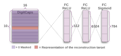
2)Decoder

As shown in the following figure from Hinton’s paper(capsule networks orignal paper), The decoder is made of three fully-connected, linear layers. The first layer sees the 10, 16-dimensional output vectors from the digit capsule layer and produces hidden_dim=512 number of outputs. The next hidden layer = 1024 , and the third and final linear layer produces an output of 784 values which is a 28x28 image!

image-center

    class Decoder(nn.Module):

        def __init__(self, input_vector_length=16, input_capsules=10, hidden_dim=512):
            '''Constructs an series of linear layers + activations.
               param input_vector_length: dimension of input capsule vector, default value = 16
               param input_capsules: number of capsules in previous layer, default value = 10
               param hidden_dim: dimensions of hidden layers, default value = 512
               '''
            super(Decoder, self).__init__()

            # calculate input_dim
            input_dim = input_vector_length * input_capsules

            # define linear layers + activations
            self.linear_layers = nn.Sequential(
                nn.Linear(input_dim, hidden_dim), # first hidden layer
                nn.ReLU(inplace=True),
                nn.Linear(hidden_dim, hidden_dim*2), # second, twice as deep
                nn.ReLU(inplace=True),
                nn.Linear(hidden_dim*2, 28*28), # can be reshaped into 28*28 image
                nn.Sigmoid() # sigmoid activation to get output pixel values in a range from 0-1
                )

        def forward(self, x):
            '''Defines the feedforward behavior.
               param x: the input; vectors from the previous DigitCaps layer
               return: two things, reconstructed images and the class scores, y
               '''
            classes = (x ** 2).sum(dim=-1) ** 0.5
            classes = F.softmax(classes, dim=-1)

            # find the capsule with the maximum vector length
            # here, vector length indicates the probability of a class' existence
            _, max_length_indices = classes.max(dim=1)

            # create a sparse class matrix
            sparse_matrix = torch.eye(10) # 10 is the number of classes
            if TRAIN_ON_GPU:
                sparse_matrix = sparse_matrix.cuda()
            # get the class scores from the "correct" capsule
            y = sparse_matrix.index_select(dim=0, index=max_length_indices.data)

            # create reconstructed pixels
            x = x * y[:, :, None]
            # flatten image into a vector shape (batch_size, vector_dim)
            flattened_x = x.contiguous().view(x.size(0), -1)
            # create reconstructed image vectors
            reconstructions = self.linear_layers(flattened_x)

            # return reconstructions and the class scores, y
            return reconstructions, y

Now let us collect all these layers (classes that we have created i.e ConvLayer,PrimaryCaps,DigitCaps,Decoder) in one class called CapsuleNetwork.

    # instantiate and print net
    capsule_net = CapsuleNetwork()

    print(capsule_net)

    # move model to GPU, if available
    if TRAIN_ON_GPU:
        capsule_net = capsule_net.cuda()

Margin Loss

Margin Loss is a classification loss (we can think of it as cross entropy) which is based on the length of the output vectors coming from the DigitCaps layer.

so let us try to elaborate it more on our example.Let us say we have an output vector called (x) coming from the digitcap layer, this ouput vector represents a certain digit from 0 to 9 as we are using MNIST. Then we will square the length(take the square root of the squared value) of the corresponding output vector of that digit capsule \(v_k = \sqrt{x^2}\) . The right capsule should have an output vector of greater than or equal 0.9 (\(v_k >=0.9\)) value while other capsules should output of smaller than or eqaul 0.1( \(v_k<=0.1\) ).

So, if we have an input image of a 0, then the “correct,” zero-detecting, digit capsule should output a vector of magnitude 0.9 or greater! For all the other digits (1-9, in this example) the corresponding digit capsule output vectors should have a magnitude that is 0.1 or less.

The following function is used to calculate the margin loss as it sums both sides of the 0.9 and 0.1 and k is the digit capsule.

image-center

where(\(T_k = 1\)) if a digit of class k is present and \(m^{+}\) = 0.9 and \(m^{-}\) = 0.1. The λ down-weighting of the loss for absent digit classes stops the initial learning from shrinking the lengths of the activity vectors of all the digit capsules. In the paper they have choosen λ = 0.5.

Note :

The total loss is simply the sum of the losses of all digit capsules.

Now we have to call the custom loss class we have implemented and we will use Adam optimizer as in the paper.

import torch.optim as optim

# custom loss
criterion = CapsuleLoss()

# Adam optimizer with default params
optimizer = optim.Adam(capsule_net.parameters())

Train the network

So the normal steps to do the training from a batch of data:

Clear the gradients of all optimized variables, by making them zero.
Forward pass: compute predicted outputs by passing inputs to the model.
Calculate the loss .
Backward pass: compute gradient of the loss with respect to model parameters.
Perform a single optimization step (parameter update).
Update average training loss .

Note

In this blog post i will not go through the train and test function as they are straight forward and they are slightly the same steps as training any network , but i will leave the implemented code in this link.

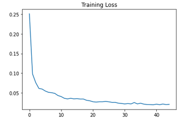
As shown in the following graph, the training loss is decreasing till 0.020.

image-center

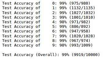
Test the network

I have tested the trained network on unseen data, and I had a good results.

image-center

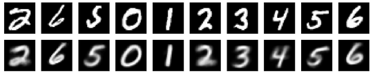
And these are the reconstructed images.

alt

For the complete code please check my github repository my github repository

References :

https://arxiv.org/pdf/1710.09829.pdf
https://cezannec.github.io/Capsule_Networks/
https://kndrck.co/posts/capsule_networks_explained/
https://github.com/cezannec/capsule_net_pytorch/blob/master/Capsule_Network.ipynb
https://www.youtube.com/watch?v=1dIEyZuZui0

Share on

Twitter Facebook Google+ LinkedIn

Nour

Simple explanation for Capsule Network with Pytoch implementation

Capsule Network

what are capsules?

What advantages does it have compared to Convolutional Neural Network(CNN)?

Model Architecture

1)Encoder

A)The convolutional layer

B)Primary capsules

C)Digit Capsules

Dynamic Routing

Dynamic Routing Algorithm

2)Decoder

Margin Loss

Train the network

Test the network

References :

Share on

You May Also Enjoy

Simple explanation for Capsule Network with Pytoch implementation